Tutorial
For this introduction to LFA Lab, we assume that you have successfully installed our software. (If this is not the case, see Installation). We start with a simple example.
The Jacobi Method
For the beginning we start with the Jacobi method applied to the Poisson equation (see Poisson Equation). The following example uses LFA Lab to compute spectral radius of the error propagator of the method.
from lfa_lab import *

# Create a 2D grid with step-size (1/32, 1/32).
fine = Grid(2, [1.0/32, 1.0/32])

# Create a poisson operator.
L = gallery.poisson_2d(fine)

# Create the jacobi smoother for L.
S = jacobi(L, 0.8)

# Compute the symbol of S.
symbol = S.symbol()

# Print spectral radius of S.
print((symbol.spectral_radius()))
Let us walk through this example step by step. To make any analysis, we first
have to define a grid, i.e., create an instance of
lfa_kernel.Grid, because all operators that we can analyze by LFA
must be defined on a grid.
Then, we can create the operator corresponding to the Poisson equation. We
call the function lfa_lab.gallery.poisson_2d() for this purpose. The
module lfa_lab.gallery contains further predefined operators that
you can use.
In the next step, we create the error propagator of the Jacobi method for the
Poisson equation, using the lfa_lab.smoother.jacobi() function. This
function can only be used with operators that are defined by a stencil. How to
define such an operator will be discussed in the section
Defining Stencil Operators.
The symbol of the error propagation operator of the Jacobi method is then
computed. Note, that this is the point where the actual computation happens,
all other operations before the computation of the symbol are merely
definitions. Since the computation of the symbol can be quite expensive, you
should store the symbol, when you want to investigate multiple of its
properties. (For the properties of a symbol, see
lfa_kernel.Symbol.)
The last step is, to compute the spectral radius of the error propagation operator. This command will output a value of 0.996 for the spectral radius.
Plotting Symbols
The Fourier symbol \(\hat{s}\) of the operator \(S\) is a description of the operator \(S\). The symbol assigns every value from \([0, \tfrac{2\pi}{h_1}) \times \cdots \times [0, \tfrac{2\pi}{h_d})\) a complex number, such that the following holds. If \(\hat{u}\) and \(\hat{f}\) are the discrete time Fourier transforms of the functions \(u\) and \(f\), respectively, and \(f = S u\) then
(pointwise multiplication). Hence, by plotting the symbol of an operator we can impove out understanding of the corresponding operator.
The following code plots the Fourer symbol of the error propagator of the Jacobi method for the discrete Poisson equation.
from lfa_lab import *
# To plot a symbol, we need to import matplotlib
import matplotlib.pyplot as mpp

fine = Grid(2, [1.0/32, 1.0/32])
L = gallery.poisson_2d(fine)
S = jacobi(L, 0.8)
symbol = S.symbol()

# Plot the symbol
plot.plot_2d(symbol)

# Tell matplotlib to show the plot.
mpp.show()
This code is just a modification to the example from the previous section. To
plot the symbol, we import the Matplotlib library. To plot the symbol
we use the function lfa_lab.plot.plot_2d(). (This function works only
for 2D problems. Problems in 1D should use the function
lfa_lab.plot.plot_2d().) To actually display the plot, we need to use
the function show() of Matplotlib. The result is shown below.
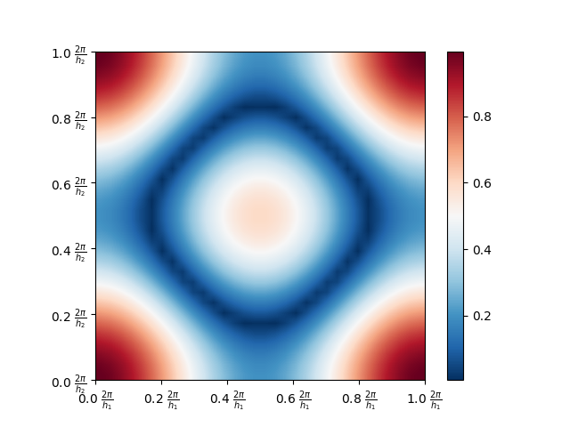
Note that LFA Lab uses the Frequency domain \([0, \tfrac{2\pi}{h_1}) \times \cdots \times [0, \tfrac{2\pi}{h_d})\). This choice implies that the low modes are located near the corners of the plot. (Recall that every mode that is node a low mode is called a high mode).
By inspecting the plot and using the relation \(\hat{f} = \hat{s} \cdot \hat{u}\), we see that applying the operator \(S\) returns a function that, in comparison to the input functions, has smaller function values on the high modes. Hence, after some applications of \(S\) the low modes will be dominating.
It is known that a function whose discrete time Fourier transform is dominant in the low modes is slowly varying. Thus, multiple applications of \(S\) result in a function which is slowly varying. Therefore, the Jacobi method is a smoother for the discrete Poisson equation.
Smoothing Analysis
The smoothing effect of an operator \(S\) can be quantified by a so called smoothing analysis. The idea of this analysis is to choose a filtering operator \(Z\) that maps the low modes to zero while leaving the high modes unchanged. (An operator like that is also called an idealized coarse grid correction.) Then, \(ZS\) characterizes how \(S\) acts on the high modes. Hence, the smoothing effect of the operator \(ZS\) is quantified by computing the spectral radius
The following code performs this computation.
from lfa_lab import *

fine = Grid(2, [1.0/32, 1.0/32])

# Create a coarse grid by selecting every second point in the x- and every
# second point in the y-direction.
coarse = fine.coarse((2,2))

L = gallery.poisson_2d(fine)
S = jacobi(L, 0.8)

# Create the filtering operator.
F = operator.hp_filter(fine, coarse)

# Apply the filter to the smoother. After applying smoother all low modes are
# removed from the spectrum.
E = F * S

print((E.symbol().spectral_radius()))
Note, a smoothing analysis can directly be performed by using the convenience
function lfa_lab.analysis.smoothing_factor().
Two Grids
The two-grid method requires
a smoothing operator \(S\) and
a coarse grid correction \(E_\mathrm{cgc}\).
The error propagator of the two-grid method is the given by
To construct the coarse grid correction error propagator we need
the linear system operator of the fine grid L,
the linear system operator of the coarse grid Lc,
the restriction operator R, and
the interpolation operator P.
This error propagator can be computed using the
lfa_lab.two_grid.coarse_grid_correction() function. This function
does nothing more than to evaluate the formula (see
Coarse Grid Correction) for the coarse grid correction. It is,
however, better to use the predefined function in LFA lab to avoid typos.
The following code computes the required operators, then the error propagator of the coarse grid correction, and then the error propagator of the entire two-grid method.
from lfa_lab import *

fine = Grid(2, [1.0/32, 1.0/32])
coarse = fine.coarse((2,2))

L = gallery.poisson_2d(fine)
Lc = gallery.poisson_2d(coarse)
S = jacobi(L, 0.8)

# Create restriction and interpolation operators.
R = gallery.fw_restriction(fine, coarse)
P = gallery.ml_interpolation(fine, coarse)

# Construct the coarse grid correction from the individual operators.
cgc = coarse_grid_correction(
        operator = L,
        coarse_operator = Lc,
        interpolation = P,
        restriction = R)

# Apply one pre- and one post-smoothing step.
E = S * cgc * S

print((E.symbol().spectral_radius()))
Defining Stencil Operators
Up to this point we used the functions from the
lfa_lab.gallery module, to create different operators. We shall now
discuss how to define these operators manually.
Let us start with the Laplace operator.
The stencil of the discrete Laplace operator is
In LFA Lab stencils are described by a list containing stencil entries. Each stencil entry is a tuple consisting of the offset of the entry and the coefficient of the entry:
[ ((o1_x, o1_y, ...), v1), ((o2_x, o2_y, ...), v2), ... ]
Using the lfa_lab.operator.from_stencil() function, we can turn this
description of a stencil into an operator that we can use in our analysis. The
following code constructs the stencil for the discrete Laplace operator:
h1 = 1.0/32
h2 = 1.0/32
entries = [
    (( 0, -1), -1.0 / (h2*h2)),
    ((-1,  0), -1.0 / (h1*h1)),
    (( 0,  0),  2.0 / (h1*h1) + 2.0 / (h2*h2)),
    (( 1,  0), -1.0 / (h1*h1)),
    (( 0,  1), -1.0 / (h2*h2))
  ]
L = operator.from_stencil(entries, grid)
Defining an interpolation and restriction operator is slightly more complicated.
A stencil operator defined using lfa_lab.operator.from_stencil() maps
from a grid with a step-size \(\mathbf{h}\) to a grid with the same
step-size \(\mathbf{h}\). Combining a stencil operator with a canonical
injection or canonical restriction (see Injection Restriction and
Injection Interpolation), however, is usually sufficient
to define the desired interpolation or restriction operator.
More precisely, to define an interpolation operator we usually combine a stencil operator \(P_\mathrm{st}\) and the injection interpolation \(P_\mathrm{inj}\) to define the desired interpolation by
Furthermore, to define a restriction operator we usually combin a stencil operator \(R_\mathrm{st}\) and the injection restriction \(R_\mathrm{inj}\) to define the destired restriction by
For example to construct the linear interpolation with standard coarsening in 2D we can use the following code:
entries = [
    ((-1, -1), 1.0/4),
    (( 0, -1), 1.0/2),
    (( 1, -1), 1.0/4),
    ((-1,  0), 1.0/2),
    (( 0,  0), 1.0),
    (( 1,  0), 1.0/2),
    ((-1,  1), 1.0/4),
    (( 0,  1), 1.0/2),
    (( 1,  1), 1.0/4),
  ]
P = operator.from_stencil(entries, fine) * \
        operator.injection_interpolation(fine, coarse)
We give below a complete example for user defined stencils.
from lfa_lab import *

fine = Grid(2, [1.0/32, 1.0/32])
coarse = fine.coarse((2,2))

# A simple function that computes the poisson stencil for a given grid.
def my_poisson_2d(grid):
    h1, h2 = grid.step_size()
    entries = [
        (( 0, -1), -1.0 / (h2*h2)),
        ((-1,  0), -1.0 / (h1*h1)),
        (( 0,  0),  2.0 / (h1*h1) + 2.0 / (h2*h2)),
        (( 1,  0), -1.0 / (h1*h1)),
        (( 0,  1), -1.0 / (h2*h2))
      ]
    return operator.from_stencil(entries, grid)

L = my_poisson_2d(fine)
Lc = my_poisson_2d(coarse)
S = jacobi(L, 0.8)

# Create the restriction operator
entries = [
    ((-1, -1), 1.0/16),
    (( 0, -1), 1.0/8),
    (( 1, -1), 1.0/16),
    ((-1,  0), 1.0/8),
    (( 0,  0), 1.0/4),
    (( 1,  0), 1.0/8),
    ((-1,  1), 1.0/16),
    (( 0,  1), 1.0/8),
    (( 1,  1), 1.0/16),
]
R = operator.injection_restriction(fine, coarse) * \
        operator.from_stencil(entries, fine)

# Create the interpolation operator.
entries = [
    ((-1, -1), 1.0/4),
    (( 0, -1), 1.0/2),
    (( 1, -1), 1.0/4),
    ((-1,  0), 1.0/2),
    (( 0,  0), 1.0),
    (( 1,  0), 1.0/2),
    ((-1,  1), 1.0/4),
    (( 0,  1), 1.0/2),
    (( 1,  1), 1.0/4),
  ]
P = operator.from_stencil(entries, fine) * \
        operator.injection_interpolation(fine, coarse)

cgc = coarse_grid_correction(
        operator = L,
        coarse_operator = Lc,
        interpolation = P,
        restriction = R)
E = S * cgc * S

print((E.symbol().spectral_radius()))
Multigrid Method
To define the error propagation operator of a multigrid method, we use the
coarse_error argument of the
lfa_lab.twogrid.coarse_grid_correction() function. This argument
gives the error propagator of the coarse grid solver. Hence, we can write a
recursive function that computes the error propagator of the multigrid method.
from lfa_lab import *

def multigrid(level, fine_grid):
    """Return a tuple consisting of the error propagation operator and the
    linear system operator of a multigrid method."""
    L = gallery.poisson_2d(fine_grid)

    if level == 1:
        # Solve exactly on the coarsest grid, hence return the zero operator.
        E = operator.zero(fine_grid)
        return (E, L)
    else:
        coarse_grid = fine_grid.coarse((2,2))
        Ec, Lc = multigrid(level-1, coarse_grid)

        S = jacobi(L, 0.8)

        R = gallery.fw_restriction(fine_grid, coarse_grid)
        P = gallery.ml_interpolation(fine_grid, coarse_grid)

        cgc = coarse_grid_correction(
                operator = L,
                coarse_operator = Lc,
                interpolation = P,
                restriction = R,
                coarse_error = Ec)

        # Apply one pre- and one post-smoothing step.
        E = S * cgc * S

        return (E, L)

# Compute error propagation operator of a three-grid method
fine_grid = Grid(2, [1.0/32, 1.0/32])
E, L = multigrid(3, fine_grid)

print((E.symbol().spectral_radius()))